WinReal3D
software for modeling of acoustic systems
Version
2.2
Alexander Yu. Sokolov
D.Sc,
Email to: [email protected]
Download program:
http://members.fortunecity.com/winreal3d/winreal3d.rar
- Introduction
Working in physics field and having made a lot of
numerical simulations of shock waves, gas-dynamical and plasma flows I decided to use this knowledge
for speaker modeling. Indeed, the propagation of sound is governed by
well-known equations. Constantly
growing power of modern PC was always attracting me to the problem of speaker
analysis.
What You find here is my attempt to represent
approach based on 3D wave simulations to speaker analysis. Several years ago I
became an enthusiast of DIY-audio (and
tubes) and decided to start this project.
This program is completely free, my idea is to have
feedback from users and same audio enthusiasts as me, this will also motivate
my future ideas. I understand this approach is quite complicated, there
are some simplifications and
restrictions (i.e. wall reflections), so more people and more ideas the
better. Send me You questions,
suggestions, the speaker enclosures You want to see included into my program.
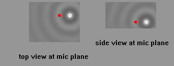
This tool allows for modeling of various speaker
enclosures taking into account the location in room as well as reflections on
the walls. Dimensions of room and speaker are linked to numerical grid
(pixels). Next figure demonstrates main dimensions, i.e. room may have
dimensions 5 х 4 х 2.6 m which in pixels becomes X1 x X2 x X3 = 125 x
80 x 52, one pixel equals 5 cm. The position of the speaker inside room is also
set, i.e. r=1 m, e=1 m, microphone is placed
at distance l=1 m in front of
driver.
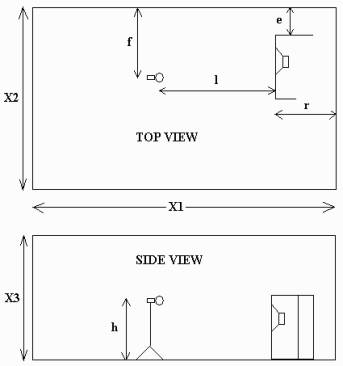
Fig. Position of the speaker and measuring
microphone in the room
- Calculation
model
The
model is based on finite difference method for numerical integration of
differential 3D wave equation, taking into account the boundary conditions on
the speaker surfaces and room walls (as well as ceiling and floor).
The driver model uses TS-parameters,
the calculation is carried out based on Newton equation of motion. Particular
pressure values on both sides of the diffuser are accounted for calculation of
diffuser acceleration. The source amplifier can have finite (nonzero) value of
output resistance.
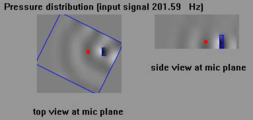
Next figures demonstrate
typical 3D solutions of pressure
distribution in the room.
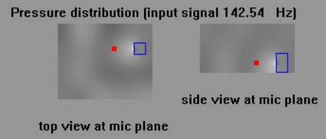
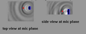
Fig.
Speaker of closed box type. The pressure distribution in the room, frequency
143 Hz.
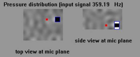
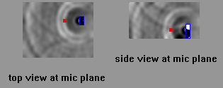
Fig.
Speaker of closed box type. The pressure distribution in the room, frequency
359 Hz.
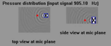
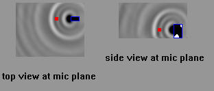
Fig.
Speaker of closed box type. The pressure distribution in the room, frequency
905 Hz.
- Various
types of acoustic enclosures
At present the following enclosures
are included into the tool:
-
ideal point source (this is useful for checking the model as well as
analysis of room modes)
-
folded
baffle with single driver
-
folded
baffle with two drivers
-
closed
(sealed) box
-
rear
opened box
-
sealed
sphere
-
transmission
line
-
transmission line 2 (folded)
-
Voight
pipe
-
Onken
-
Bass
reflex
-
TQWP
-
Back
loaded horn (BLH)
Note: for Onken, bass reflex and BLH the inner channels (ports) must be wider than the grid size, at least two pixels are necessary to represent the channel width. Thus, it is recommended to reduce the grid as much as possible for these enclosures.
- Presentation
of results
There are the following features of the
software:
-
Simulation
with given frequency. This is useful for visual analysis and better
understanding of acoustic wave
propagation in the room;
-
Scanning
of all frequencies. In this mode the frequency is gradually increased from
minimum to maximum value, and the pressure level is determined at the measuring
point. Such calculation takes much time as it is necessary to run each frequency
for several hundred of milliseconds;
-
Fourier
spectral analysis.
Fourier
analysis is the most convenient and allows for calculation of amplitude and
phase response at once. It is recommended to set integration (measuring) time
of about 500 milliseconds or more for Fourier analysis.
- How
to start
-
Run
WinReal3D
-
In
menu “Action” use “Open Project” and select file “demo_project”.
Now the
demo project is loaded and one can calculate frequency response.
These are
several notes about the program:
All parameter are given in menu “Parameters”
which includes:
1 “Driver” is used for driver parameters
setting. “Calculate” helps to translate TS parameters into mass, compliance
etc.
1.2 “Room” is used to set the room geometry and speaker and microphone position.
All dimensions are given in pixels. By default 1 pixel = 5 cm. Grid size can be
changed in “Grid size” menu.
1.3 “Speaker” is used for selecting from various types of enclosures. Mark “use
this enclosure” to activate the selected type. The project file stores all
enclosures such that they can be considered and compared to each other during one session of work.
1.4 “Input” is used to set input voltage, amplifier resistance and the type of
the signal: pure sine wave or pink noise (central frequency with side
harmonics). It is advised to selected the sine wave.
Remark: The pink noise can be used only in “Sim one frequency” or “Scan frequencies”
1.5
“Duration” is used for setting of measuring time. Microphone has to be switch
on after the first wave arrives to the microphone from the speaker, thus is it
convenient to set this time as a distance (i.e. distance to the speaker)
divided by sonic velocity Vs. The second time (switch off) is determined also
as a typical distance divide by Vs. It is advised to select the measuring time
(difference between mic on and mic off)
of the value of 500 millisec or more.
1.6
“Reflection on Walls” is used for setting the reflection coefficients on walls,
floor and ceiling.
Remark:
If the room is rotated (see “Rotate room”) only K=1 is applied on side walls.
1.7 Rotate room – see below.
To start
simulation there are three actions in menu “Action”:
1. “Sim one frequency” is used to start calculation with given frequency. This shows
the structure and propagation of waves in the room. The values below the output
window provide SPL for this frequency which was set in “Input” menu. If “wave
packet” was selected SPL regards to this.
2. “Scan Frequencies”: this option automatically starts the scanning of all
frequencies, that is low frequency is calculated at first, then the frequency is increased and so on. At the end
SPL plot is shown. Each frequency is calculated for the measuring time determined
in “Input”. This option requires considerable amount of time.
3. “Fourier” option is for Fourier analysis. IT IS RECOMMENDED TO START WITH
THIS OPTION. Fourier includes calculation of one, two frequencies or white
noise. Select “white noise” for calculation of amplitude and phase response.
For Fourier analysis set the measuring time of about 500 millisec ore even
more, see below.
- Accuracy
of Fourier Analysis
To
understand the accuracy of Fourier analysis let us set all reflection
coefficients to zero (K=0). This
arrives us to the model of “no-echo” camera. In the model the walls are
acoustically transparent which is done via the corresponding boundary
conditions on the room surfaces. It is difficult to completely eliminate the
reflections in numerical model, however, the reflecting waves are relatively
small as it is seen from the examples below.
Sine wave from ideal point source in “no-echo”
camera.
The next
figures shows the spectrums of ideal point source in “no-echo” camera in the
range of 20-1000 Hz. The higher measuring time the better accuracy. Especially
low frequency range requires sufficient averaging time as the period of wave is
large.
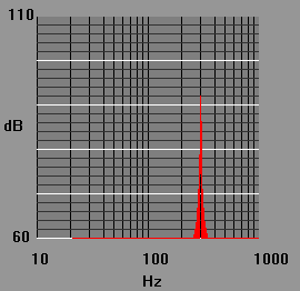
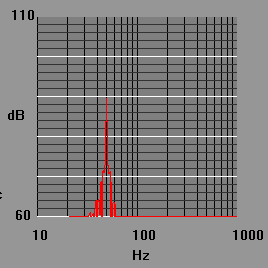
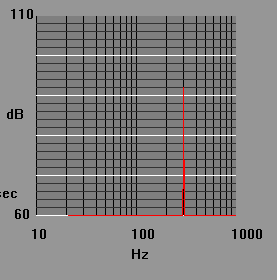
6.1 Measuring time 300 ms
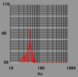
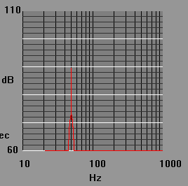
Spectrum of original signal 50 Hz
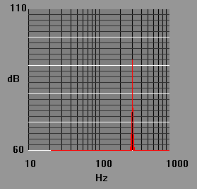
Spectrum of original signal 300 Hz
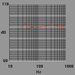
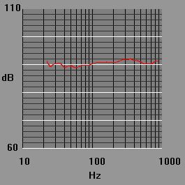
Spectrum of while noise
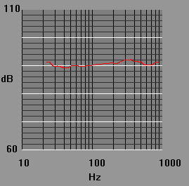
6.2 Measuring time 600 ms.
Spectrum of original signal 50 Hz
Spectrum of original signal 600 Hz
Spectrum of white noise
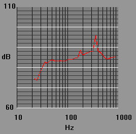
6.3 Measuring time 1200 ms (1.2 s).
Spectrum of original signal 50 Hz
Spectrum of original signal 300 Hz
Spectrum of white noise
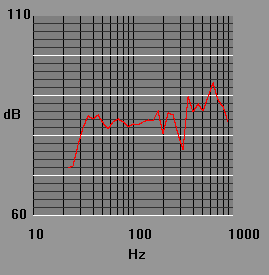
Thus, for measuring times of the order of 0.5 sec or more the reasonable accuracy is achieved. At middle frequencies there is a small gain (+ 2dB). In principle this peak can be taken into account as the correction parameter for real speaker calculation (similar to correction curve of real measuring microphone).
7
Some
examples: Closed (sealed) box
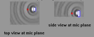
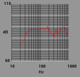
Fig. Set initially box dimensions as W х H х D=0.6 х 1 х 0.3 m (the wider side panel forward), V=160
liters. The driver is placed at 0.6 m from floor. Set reflection coefficients
K=0, that is no-echo camera. The driver is 12 inch JBL123-A, the amplifier has
R=2.5 ohm.
SPL in no-echo camera, measuring time 0.6 s.
Next we
add reflections from the floor only (K=1). The other room surfaces are
acoustically transparent. As it is seen SPL is increased by 3dB in low range
(which is in theoretical agreement), however, the middle range is dropped (And
one may think that is would be wise to play with soft carpet in from of the
speaker to obtain the middle curve of two plots!)
SPL with reflection from the floor only. t=0.6
s..
Next, let
us run the similar simulation but with all reflection surfaces having K=0.8.
The SPL curve remains same “eye-pleasant”.

SPL with all room surfaces having K=0.8, t=0.6
s.
For the
sake if interest let us rotate the speaker such that the narrow side of the box
is in the front (narrow side toward the mic). At first we look at the SPL in
“no-echo” camera:
Too lack
of bass we have!
SPL for same volume of closed box but the
narrow side is in the front, t=0.6 s, no-echo camera.
Switching
on the reflection from the floor (K=1):
Same but with the reflection form the floor
K=1, t=0.6 s.
Finally
switch on all reflections from walls, floor and ceiling (К=0.8):
SPL of front narrow side speaker, K=0.8, t= 0.6
s
9. Rotation of speaker with respect
to the room
This tool allows to place the speaker with the
driver directed towards the center of the room, which is commonly used in
reality. See the fig. below:
The angle
of rotation is set in menu “Rotate
Room”.
Remark.
When this option is used only full reflections on side walls (K=1) is used in
the current version.
Remark
2. Calculation of room with rotations is slower than simple straight room.
Open
project demo_rotated for
modeling of room with rotation.
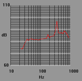
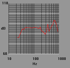
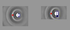
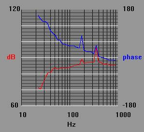
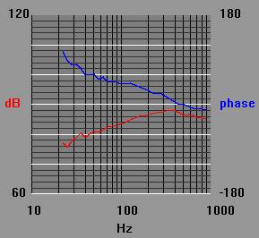
10. Effect of internal box waves
This tool
allows for accounting of the effect of internal box modes. Next figures show
the calculated amplitude and phase responses under two conditions: (left)
taking into account the effect of pressure at the internal surface on driver
diaphragm motion and (right) neglecting by this effect. In the second case it
is assumed that pressure disturbances near the diaphragm are zero inside the
box. The speaker has dimensions of 1 x 0.5 x 0.3 m, such that the own box
frequencies (half wavelength equals distance between walls) are
170 Hz, 340 Hz and 570 Hz. The
integral behavior of the speaker exhibits two peaks at 170 and 340 Hz, and the
third resonance is negligible.
11. Concluding remarks
As I
already mentioned at the beginning this is an open project. One person cannot compare
numerical model with all enclosures. If You find this program useful, write to
me, if You suggest any improvements other users will also appreciate this.